The purpose of this post is to report an erratum to the 2012 paper “An inverse theorem for the Gowers -norm” of Ben Green, myself, and Tamar Ziegler (previously discussed in this blog post). The main results of this paper have been superseded with stronger quantitative results, first in work of Manners (using somewhat different methods), and more recently in a remarkable paper of Leng, Sah, and Sawhney which combined the methods of our paper with several new innovations to obtain quite strong bounds (of quasipolynomial type); see also an alternate proof of our main results (again by quite different methods) by Candela and Szegedy. In the course of their work, they discovered some fixable but nontrivial errors in our paper. These (rather technical) issues were already implicitly corrected in this followup work which supersedes our own paper, but for the sake of completeness we are also providing a formal erratum for our original paper, which can be found here. We thank Leng, Sah, and Sawhney for bringing these issues to our attention.
Excluding some minor (mostly typographical) issues which we also have reported in this erratum, the main issues stemmed from a conflation of two notions of a degree filtration
of a group , which is a nested sequence of subgroups that obey the relation for all . The weaker notion (sometimes known as a prefiltration) permits the group to be strictly smaller than , while the stronger notion requires and to equal. In practice, one can often move between the two concepts, as is always normal in , and a prefiltration behaves like a filtration on every coset of (after applying a translation and perhaps also a conjugation). However, we did not clarify this issue sufficiently in the paper, and there are some places in the text where results that were only proven for filtrations were applied for prefiltrations. The erratum fixes this issues, mostly by clarifying that we work with filtrations throughout (which requires some decomposition into cosets in places where prefiltrations are generated). Similar adjustments need to be made for multidegree filtrations and degree-rank filtrations, which we also use heavily on our paper.
In most cases, fixing this issue only required minor changes to the text, but there is one place (Section 8) where there was a non-trivial problem: we used the claim that the final group was a central group, which is true for filtrations, but not necessarily for prefiltrations. This fact (or more precisely, a multidegree variant of it) was used to claim a factorization for a certain product of nilcharacters, which is in fact not true as stated. In the erratum, a substitute factorization for a slightly different product of nilcharacters is provided, which is still sufficient to conclude the main result of this part of the paper (namely, a statistical linearization of a certain family of nilcharacters in the shift parameter ).
Again, we stress that these issues do not impact the paper of Leng, Sah, and Sawhney, as they adapted the methods in our paper in a fashion that avoids these errors.
where the supremum is over all Følner sequences of . Given a set in , we define the restricted sumset to be the set of all pairs where are distinct elements of .
Theorem 1 Let be a countably infinite abelian group with the index finite. Let be a positive Banach density subset of . Then there exists an infinite set and such that .
Strictly speaking, the main result of Kra et al. only claims this theorem for the case of the integers , but as noted in the recent preprint of Charamaras and Mountakis, the argument in fact applies for all countable abelian in which the subgroup has finite index. This condition is in fact necessary (as observed by forthcoming work of Ethan Acklesberg): if has infinite index, then one can find a subgroup of of index for any that contains (or equivalently, is -torsion). If one lets be an enumeration of , and one can then check that the set
has positive Banach density, but does not contain any set of the form for any (indeed, from the pigeonhole principle and the -torsion nature of one can show that must intersect whenever has cardinality larger than ). It is also necessary to work with restricted sums rather than full sums : a counterexample to the latter is provided for instance by the example with and . Finally, the presence of the shift is also necessary, as can be seen by considering the example of being the odd numbers in , though in the case one can of course delete the shift at the cost of giving up the containment .
Theorem 1 resembles other theorems in density Ramsey theory, such as Szemerédi’s theorem, but with the notable difference that the pattern located in the dense set is infinite rather than merely arbitrarily large but finite. As such, it does not seem that this theorem can be proven by purely finitary means. However, one can view this result as the conjunction of an infinite number of statements, each of which is a finitary density Ramsey theory statement. To see this, we need some more notation. Observe from Tychonoff’s theorem that the collection is a compact topological space (with the topology of pointwise convergence) (it is also metrizable since is countable). Subsets of can be thought of as properties of subsets of ; for instance, the property a subset of of being finite is of this form, as is the complementary property of being infinite. A property of subsets of can then be said to be closed or open if it corresponds to a closed or open subset of . Thus, a property is closed and only if if it is closed under pointwise limits, and a property is open if, whenever a set has this property, then any other set that shares a sufficiently large (but finite) initial segment with will also have this property. Since is compact and Hausdorff, a property is closed if and only if it is compact.
The properties of being finite or infinite are neither closed nor open. Define a smallness property to be a closed (or compact) property of subsets of that is only satisfied by finite sets; the complement to this is a largeness property, which is an open property of subsets of that is satisfied by all infinite sets. (One could also choose to impose other axioms on these properties, for instance requiring a largeness property to be an upper set, but we will not do so here.) Examples of largeness properties for a subset of include:
has at least elements.
is non-empty and has at least elements, where is the smallest element of .
is non-empty and has at least elements, where is the element of .
halts when given as input, where is a given Turing machine that halts whenever given an infinite set as input. (Note that this encompasses the preceding three examples as special cases, by selecting appropriately.)
We will call a set obeying a largeness property an -large set.
Theorem 1 is then equivalent to the following “almost finitary” version (cf. this previous discussion of almost finitary versions of the infinite pigeonhole principle):
Theorem 2 (Almost finitary form of main theorem) Let be a countably infinite abelian group with finite. Let be a Følner sequence in , let , and let be a largeness property for each . Then there exists such that if is such that for all , then there exists a shift and contains a -large set such that .
Proof of Theorem 2 assuming Theorem 1. Let , , be as in Theorem 2. Suppose for contradiction that Theorem 2 failed, then for each we can find with for all , such that there is no and -large such that . By compactness, a subsequence of the converges pointwise to a set , which then has Banach density at least . By Theorem 1, there is an infinite set and a such that . By openness, we conclude that there exists a finite -large set contained in , thus . This implies that for infinitely many , a contradiction.
Proof of Theorem 1 assuming Theorem 2. Let be as in Theorem 1. If the claim failed, then for each , the property of being a set for which would be a smallness property. By Theorem 2, we see that there is a and a obeying the complement of this property such that , a contradiction.
Remark 3 Define a relation between and by declaring if and . The key observation that makes the above equivalences work is that this relation is continuous in the sense that if is an open subset of , then the inverse image
is also open. Indeed, if for some , then contains a finite set such that , and then any that contains both and lies in .
For each specific largeness property, such as the examples listed previously, Theorem 2 can be viewed as a finitary assertion (at least if the property is “computable” in some sense), but if one quantifies over all largeness properties, then the theorem becomes infinitary. In the spirit of the Paris-Harrington theorem, I would in fact expect some cases of Theorem 2 to undecidable statements of Peano arithmetic, although I do not have a rigorous proof of this assertion.
Despite the complicated finitary interpretation of this theorem, I was still interested in trying to write the proof of Theorem 1 in some sort of “pseudo-finitary” manner, in which one can see analogies with finitary arguments in additive combinatorics. The proof of Theorem 1 that I give below the fold is my attempt to achieve this, although to avoid a complete explosion of “epsilon management” I will still use at one juncture an ergodic theory reduction from the original paper of Kra et al. that relies on such infinitary tools as the ergodic decomposition, the ergodic theory, and the spectral theorem. Also some of the steps will be a little sketchy, and assume some familiarity with additive combinatorics tools (such as the arithmetic regularity lemma).
This post contains two unrelated announcements. Firstly, I would like to promote a useful list of resources for AI in Mathematics, that was initiated by Talia Ringer (with the crowdsourced assistance of many others) during the National Academies workshop on “AI in mathematical reasoning” last year. This list is now accepting new contributions, updates, or corrections; please feel free to submit them directly to the list (which I am helping Talia to edit). Incidentally, next week there will be a second followup webinar to the aforementioned workshop, building on the topics covered there. (The first webinar may be found here.)
Secondly, I would like to advertise the erdosproblems.com website, launched recently by Thomas Bloom. This is intended to be a living repository of the many mathematical problems proposed in various venues by Paul Erdős, who was particularly noted for his influential posing of such problems. For a tour of the site and an explanation of its purpose, I can recommend Thomas’s recent talk on this topic at a conference last week in honor of Timothy Gowers.
Thomas is currently issuing a call for help to develop the erdosproblems.com website in a number of ways (quoting directly from that page):
You know Github and could set a suitable project up to allow people to contribute new problems (and corrections to old ones) to the database, and could help me maintain the Github project;
You know things about web design and have suggestions for how this website could look or perform better;
You know things about Python/Flask/HTML/SQL/whatever and want to help me code cool new features on the website;
You know about accessibility and have an idea how I can make this website more accessible (to any group of people);
You are a mathematician who has thought about some of the problems here and wants to write an expanded commentary for one of them, with lots of references, comparisons to other problems, and other miscellaneous insights (mathematician here is interpreted broadly, in that if you have thought about the problems on this site and are willing to write such a commentary you qualify);
You knew Erdős and have any memories or personal correspondence concerning a particular problem;
You have solved an Erdős problem and I’ll update the website accordingly (and apologies if you solved this problem some time ago);
You have spotted a mistake, typo, or duplicate problem, or anything else that has confused you and I’ll correct things;
You are a human being with an internet connection and want to volunteer a particular Erdős paper or problem list to go through and add new problems from (please let me know before you start, to avoid duplicate efforts);
You have any other ideas or suggestions – there are probably lots of things I haven’t thought of, both in ways this site can be made better, and also what else could be done from this project. Please get in touch with any ideas!
I for instance contributed a problem to the site (#587) that Erdős himself gave to me personally (this was the topic of a somewhat well known photo of Paul and myself, and which he communicated again to be shortly afterwards on a postcard; links to both images can be found by following the above link). As it turns out, this particular problem was essentially solved in 2010 by Nguyen and Vu.
Theorem 1 (Marton’s conjecture) Let be an abelian -torsion group (thus, for all ), and let be such that . Then can be covered by at most translates of a subgroup of of cardinality at most . Moreover, is contained in for some .
We had previously established the case of this result, with the number of translates bounded by (which was subsequently improved to by Jyun-Jie Liao), but without the additional containment . It remains a challenge to replace by a bounded constant (such as ); this is essentially the “polynomial Bogolyubov conjecture”, which is still open. The result has been formalized in the proof assistant language Lean, as discussed in this previous blog post. As a consequence of this result, many of the applications of the previous theorem may now be extended from characteristic to higher characteristic.
Our proof techniques are a modification of those in our previous paper, and in particular continue to be based on the theory of Shannon entropy. For inductive purposes, it turns out to be convenient to work with the following version of the conjecture (which, up to -dependent constants, is actually equivalent to the above theorem):
Theorem 2 (Marton’s conjecture, entropy form) Let be an abelian -torsion group, and let be independent finitely supported random variables on , such that
where denotes Shannon entropy. Then there is a uniform random variable on a subgroup of such that
where denotes the entropic Ruzsa distance (see previous blog post for a definition); furthermore, if all the take values in some symmetric set , then lies in for some .
As a first approximation, one should think of all the as identically distributed, and having the uniform distribution on , as this is the case that is actually relevant for implying Theorem 1; however, the recursive nature of the proof of Theorem 2 requires one to manipulate the separately. It also is technically convenient to work with independent variables, rather than just a pair of variables as we did in the case; this is perhaps the biggest additional technical complication needed to handle higher characteristics.
The strategy, as with the previous paper, is to attempt an entropy decrement argument: to try to locate modifications of that are reasonably close (in Ruzsa distance) to the original random variables, while decrementing the “multidistance”
which turns out to be a convenient metric for progress (for instance, this quantity is non-negative, and vanishes if and only if the are all translates of a uniform random variable on a subgroup ). In the previous paper we modified the corresponding functional to minimize by some additional terms in order to improve the exponent , but as we are not attempting to completely optimize the constants, we did not do so in the current paper (and as such, our arguments here give a slightly different way of establishing the case, albeit with somewhat worse exponents).
As before, we search for such improved random variables by introducing more independent random variables – we end up taking an array of random variables for , with each a copy of , and forming various sums of these variables and conditioning them against other sums. Thanks to the magic of Shannon entropy inequalities, it turns out that it is guaranteed that at least one of these modifications will decrease the multidistance, except in an “endgame” situation in which certain random variables are nearly (conditionally) independent of each other, in the sense that certain conditional mutual informations are small. In particular, in the endgame scenario, the row sums of our array will end up being close to independent of the column sums , subject to conditioning on the total sum . Not coincidentally, this type of conditional independence phenomenon also shows up when considering row and column sums of iid independent gaussian random variables, as a specific feature of the gaussian distribution. It is related to the more familiar observation that if are two independent copies of a Gaussian random variable, then and are also independent of each other.
Up until now, the argument does not use the -torsion hypothesis, nor the fact that we work with an array of random variables as opposed to some other shape of array. But now the torsion enters in a key role, via the obvious identity
In the endgame, the any pair of these three random variables are close to independent (after conditioning on the total sum ). Applying some “entropic Ruzsa calculus” (and in particular an entropic version of the Balog–Szeméredi–Gowers inequality), one can then arrive at a new random variable of small entropic doubling that is reasonably close to all of the in Ruzsa distance, which provides the final way to reduce the multidistance.
Besides the polynomial Bogolyubov conjecture mentioned above (which we do not know how to address by entropy methods), the other natural question is to try to develop a characteristic zero version of this theory in order to establish the polynomial Freiman–Ruzsa conjecture over torsion-free groups, which in our language asserts (roughly speaking) that random variables of small entropic doubling are close (in Ruzsa distance) to a discrete Gaussian random variable, with good bounds. The above machinery is consistent with this conjecture, in that it produces lots of independent variables related to the original variable, various linear combinations of which obey the same sort of entropy estimates that gaussian random variables would exhibit, but what we are missing is a way to get back from these entropy estimates to an assertion that the random variables really are close to Gaussian in some sense. In continuous settings, Gaussians are known to extremize the entropy for a given variance, and of course we have the central limit theorem that shows that averages of random variables typically converge to a Gaussian, but it is not clear how to adapt these phenomena to the discrete Gaussian setting (without the circular reasoning of assuming the polynoimal Freiman–Ruzsa conjecture to begin with).
The first progress prize competition for the AI Mathematical Olympiad has now launched. (Disclosure: I am on the advisory committee for the prize.) This is a competition in which contestants submit an AI model which, after the submissions deadline on June 27, will be tested (on a fixed computational resource, without internet access) on a set of 50 “private” test math problems, each of which has an answer as an integer between 0 and 999. Prior to the close of submission, the models can be tested on 50 “public” test math problems (where the results of the model are public, but not the problems themselves), as well as 10 training problems that are available to all contestants. As of this time of writing, the leaderboard shows that the best-performing model has solved 4 out of 50 of the questions (a standard benchmark, Gemma 7B, had previously solved 3 out of 50). A total of $ ($1.048 million) has been allocated for various prizes associated to this competition. More detailed rules can be found here.
Let be a non-empty finite set. If is a random variable taking values in , the Shannon entropy of is defined as
There is a nice variational formula that lets one compute logs of sums of exponentials in terms of this entropy:
Lemma 1 (Gibbs variational formula) Let be a function. Then
Proof: Note that shifting by a constant affects both sides of (1) the same way, so we may normalize . Then is now the probability distribution of some random variable , and the inequality can be rewritten as
In this note I would like to use this variational formula (which is also known as the Donsker-Varadhan variational formula) to give another proof of the following inequality of Carbery.
Theorem 2 (Generalized Cauchy-Schwarz inequality) Let , let be finite non-empty sets, and let be functions for each . Let and be positive functions for each . Then
where is the quantity
where is the set of all tuples such that for .
Thus for instance, the identity is trivial for . When , the inequality reads
which is easily proven by Cauchy-Schwarz, while for the inequality reads
which can also be proven by elementary means. However even for , the existing proofs require the “tensor power trick” in order to reduce to the case when the are step functions (in which case the inequality can be proven elementarily, as discussed in the above paper of Carbery).
We now prove this inequality. We write and for some functions and . If we take logarithms in the inequality to be proven and apply Lemma 1, the inequality becomes
where ranges over random variables taking values in , range over tuples of random variables taking values in , and range over random variables taking values in . Comparing the suprema, the claim now reduces to
Lemma 3 (Conditional expectation computation) Let be an -valued random variable. Then there exists a -valued random variable , where each has the same distribution as , and
Proof: We induct on . When we just take . Now suppose that , and the claim has already been proven for , thus one has already obtained a tuple with each having the same distribution as , and
By hypothesis, has the same distribution as . For each value attained by , we can take conditionally independent copies of and conditioned to the events and respectively, and then concatenate them to form a tuple in , with a further copy of that is conditionally independent of relative to . One can the use the entropy chain rule to compute
and the claim now follows from the induction hypothesis.
With a little more effort, one can replace by a more general measure space (and use differential entropy in place of Shannon entropy), to recover Carbery’s inequality in full generality; we leave the details to the interested reader.
In my previous post, I walked through the task of formally deducing one lemma from another in Lean 4. The deduction was deliberately chosen to be short and only showcased a small number of Lean tactics. Here I would like to walk through the process I used for a slightly longer proof I worked out recently, after seeing the following challenge from Damek Davis: to formalize (in a civilized fashion) the proof of the following lemma:
Lemma. Let and be sequences of real numbers indexed by natural numbers , with non-increasing and non-negative. Suppose also that for all . Then for all .
Here I tried to draw upon the lessons I had learned from the PFR formalization project, and to first set up a human readable proof of the lemma before starting the Lean formalization – a lower-case “blueprint” rather than the fancier Blueprint used in the PFR project. The main idea of the proof here is to use the telescoping series identity
Since is non-negative, and by hypothesis, we have
but by the monotone hypothesis on the left-hand side is at least , giving the claim.
This is already a human-readable proof, but in order to formalize it more easily in Lean, I decided to rewrite it as a chain of inequalities, starting at and ending at . With a little bit of pen and paper effort, I obtained
(by field identities)
(by the formula for summing a constant)
(by the monotone hypothesis)
(by the hypothesis
(by telescoping series)
(by the non-negativity of ).
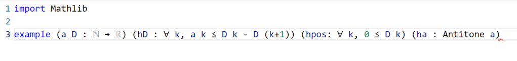
I decided that this was a good enough blueprint for me to work with. The next step is to formalize the statement of the lemma in Lean. For this quick project, it was convenient to use the online Lean playground, rather than my local IDE, so the screenshots will look a little different from those in the previous post. (If you like, you can follow this tour in that playground, by clicking on the screenshots of the Lean code.) I start by importing Lean’s math library, and starting an example of a statement to state and prove:
Now we have to declare the hypotheses and variables. The main variables here are the sequences and , which in Lean are best modeled by functions a, D from the natural numbers ℕ to the reals ℝ. (One can choose to “hardwire” the non-negativity hypothesis into the by making D take values in the nonnegative reals (denoted NNReal in Lean), but this turns out to be inconvenient, because the laws of algebra and summation that we will need are clunkier on the non-negative reals (which are not even a group) than on the reals (which are a field). So we add in the variables:
Now we add in the hypotheses, which in Lean convention are usually given names starting with h. This is fairly straightforward; the one thing is that the property of being monotone decreasing already has a name in Lean’s Mathlib, namely Antitone, and it is generally a good idea to use the Mathlib provided terminology (because that library contains a lot of useful lemmas about such terms).
One thing to note here is that Lean is quite good at filling in implied ranges of variables. Because a and D have the natural numbers ℕ as their domain, the dummy variable k in these hypotheses is automatically being quantified over ℕ. We could have made this quantification explicit if we so chose, for instance using ∀ k : ℕ, 0 ≤ D k instead of ∀ k, 0 ≤ D k, but it is not necessary to do so. Also note that Lean does not require parentheses when applying functions: we write D k here rather than D(k) (which in fact does not compile in Lean unless one puts a space between the D and the parentheses). This is slightly different from standard mathematical notation, but is not too difficult to get used to.
This looks like the end of the hypotheses, so we could now add a colon to move to the conclusion, and then add that conclusion:
This is a perfectly fine Lean statement. But it turns out that when proving a universally quantified statement such as ∀ k, a k ≤ D 0 / (k + 1), the first step is almost always to open up the quantifier to introduce the variable k (using the Lean command intro k). Because of this, it is slightly more efficient to hide the universal quantifier by placing the variable k in the hypotheses, rather than in the quantifier (in which case we have to now specify that it is a natural number, as Lean can no longer deduce this from context):
At this point Lean is complaining of an unexpected end of input: the example has been stated, but not proved. We will temporarily mollify Lean by adding a sorry as the purported proof:
Now Lean is content, other than giving a warning (as indicated by the yellow squiggle under the example) that the proof contains a sorry.
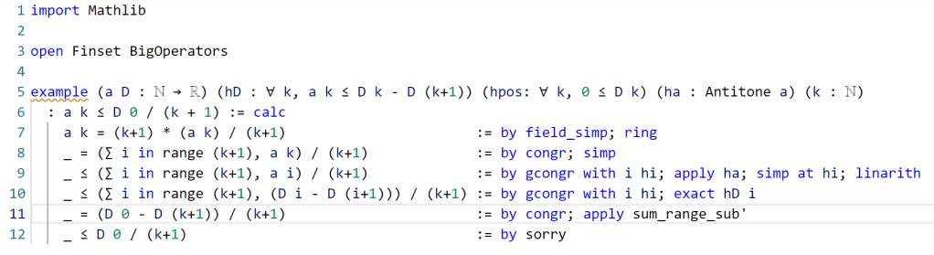
It is now time to follow the blueprint. The Lean tactic for proving an inequality via chains of other inequalities is known as calc. We use the blueprint to fill in the calc that we want, leaving the justifications of each step as “sorry”s for now:
Here, we “open“ed the Finset namespace in order to easily access Finset‘s range function, with range k basically being the finite set of natural numbers , and also “open“ed the BigOperators namespace to access the familiar ∑ notation for (finite) summation, in order to make the steps in the Lean code resemble the blueprint as much as possible. One could avoid opening these namespaces, but then expressions such as ∑ i in range (k+1), a i would instead have to be written as something like Finset.sum (Finset.range (k+1)) (fun i ↦ a i), which looks a lot less like like standard mathematical writing. The proof structure here may remind some readers of the “two column proofs” that are somewhat popular in American high school geometry classes.
Now we have six sorries to fill. Navigating to the first sorry, Lean tells us the ambient hypotheses, and the goal that we need to prove to fill that sorry:
The ⊢ symbol here is Lean’s marker for the goal. The uparrows ↑ are coercion symbols, indicating that the natural number k has to be converted to a real number in order to interact via arithmetic operations with other real numbers such as a k, but we can ignore these coercions for this tour (for this proof, it turns out Lean will basically manage them automatically without need for any explicit intervention by a human).
The goal here is a self-evident algebraic identity; it involves division, so one has to check that the denominator is non-zero, but this is self-evident. In Lean, a convenient way to establish algebraic identities is to use the tactic field_simp to clear denominators, and then ring to verify any identity that is valid for commutative rings. This works, and clears the first sorry:
field_simp, by the way, is smart enough to deduce on its own that the denominator k+1 here is manifestly non-zero (and in fact positive); no human intervention is required to point this out. Similarly for other “clearing denominator” steps that we will encounter in the other parts of the proof.
Now we navigate to the next `sorry`. Lean tells us the hypotheses and goals:
We can reduce the goal by canceling out the common denominator ↑k+1. Here we can use the handy Lean tactic congr, which tries to match two sides of an equality goal as much as possible, and leave any remaining discrepancies between the two sides as further goals to be proven. Applying congr, the goal reduces to
Here one might imagine that this is something that one can prove by induction. But this particular sort of identity – summing a constant over a finite set – is already covered by Mathlib. Indeed, searching for Finset, sum, and const soon leads us to the Finset.sum_const lemma here. But there is an even more convenient path to take here, which is to apply the powerful tactic simp, which tries to simplify the goal as much as possible using all the “simp lemmas” Mathlib has to offer (of which Finset.sum_const is an example, but there are thousands of others). As it turns out, simp completely kills off this identity, without any further human intervention:
Now we move on to the next sorry, and look at our goal:
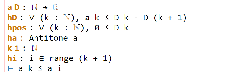
congr doesn’t work here because we have an inequality instead of an equality, but there is a powerful relative gcongr of congr that is perfectly suited for inequalities. It can also open up sums, products, and integrals, reducing global inequalities between such quantities into pointwise inequalities. If we invoke gcongr with i hi (where we tell gcongr to use i for the variable opened up, and hi for the constraint this variable will satisfy), we arrive at a greatly simplified goal (and a new ambient variable and hypothesis):
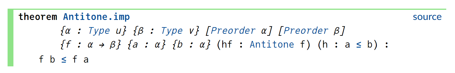
Now we need to use the monotonicity hypothesis on a, which we have named ha here. Looking at the documentation for Antitone, one finds a lemma that looks applicable here:
One can apply this lemma in this case by writing apply Antitone.imp ha, but because ha is already of type Antitone, we can abbreviate this to apply ha.imp. (Actually, as indicated in the documentation, due to the way Antitone is defined, we can even just use apply ha here.) This reduces the goal nicely:
The goal is now very close to the hypothesis hi. One could now look up the documentation for Finset.range to see how to unpack hi, but as before simp can do this for us. Invoking simp at hi, we obtain
Now the goal and hypothesis are very close indeed. Here we can just close the goal using the linarith tactic used in the previous tour:
The next sorry can be resolved by similar methods, using the hypothesis hD applied at the variable i:
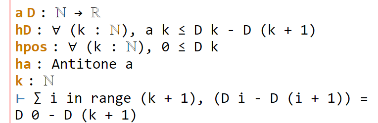
Now for the penultimate sorry. As in a previous step, we can use congr to remove the denominator, leaving us in this state:
This is a telescoping series identity. One could try to prove it by induction, or one could try to see if this identity is already in Mathlib. Searching for Finset, sum, and sub will locate the right tool (as the fifth hit), but a simpler way to proceed here is to use the exact? tactic we saw in the previous tour:
A brief check of the documentation for sum_range_sub' confirms that this is what we want. Actually we can just use apply sum_range_sub' here, as the apply tactic is smart enough to fill in the missing arguments:
One last sorry to go. As before, we use gcongr to cancel denominators, leaving us with
This looks easy, because the hypothesis hpos will tell us that D (k+1) is nonnegative; specifically, the instance hpos (k+1) of that hypothesis will state exactly this. The linarith tactic will then resolve this goal once it is told about this particular instance:
We now have a complete proof – no more yellow squiggly line in the example. There are two warnings though – there are two variables i and hi introduced in the proof that Lean’s “linter” has noticed are not actually used in the proof. So we can rename them with underscores to tell Lean that we are okay with them not being used:
This is a perfectly fine proof, but upon noticing that many of the steps are similar to each other, one can do a bit of “code golf” as in the previous tour to compactify the proof a bit:
With enough familiarity with the Lean language, this proof actually tracks quite closely with (an optimized version of) the human blueprint.
This concludes the tour of a lengthier Lean proving exercise. I am finding the pre-planning step of the proof (using an informal “blueprint” to break the proof down into extremely granular pieces) to make the formalization process significantly easier than in the past (when I often adopted a sequential process of writing one line of code at a time without first sketching out a skeleton of the argument). (The proof here took only about 15 minutes to create initially, although for this blog post I had to recreate it with screenshots and supporting links, which took significantly more time.) I believe that a realistic near-term goal for AI is to be able to fill in automatically a significant fraction of the sorts of atomic “sorry“s of the size one saw in this proof, allowing one to convert a blueprint to a formal Lean proof even more rapidly.
One final remark: in this tour I filled in the “sorry“s in the order in which they appeared, but there is actually no requirement that one does this, and once one has used a blueprint to atomize a proof into self-contained smaller pieces, one can fill them in in any order. Importantly for a group project, these micro-tasks can be parallelized, with different contributors claiming whichever “sorry” they feel they are qualified to solve, and working independently of each other. (And, because Lean can automatically verify if their proof is correct, there is no need to have a pre-existing bond of trust with these contributors in order to accept their contributions.) Furthermore, because the specification of a “sorry” someone can make a meaningful contribution to the proof by working on an extremely localized component of it without needing the mathematical expertise to understand the global argument. This is not particularly important in this simple case, where the entire lemma is not too hard to understand to a trained mathematician, but can become quite relevant for complex formalization projects.
Since the release of my preprint with Tim, Ben, and Freddie proving the Polynomial Freiman-Ruzsa (PFR) conjecture over , I (together with Yael Dillies and Bhavik Mehta) have started a collaborative project to formalize this argument in the proof assistant language Lean4. It has been less than a week since the project was launched, but it is proceeding quite well, with a significant fraction of the paper already either fully or partially formalized. The project has been greatly assisted by the Blueprint tool of Patrick Massot, which allows one to write a human-readable “blueprint” of the proof that is linked to the Lean formalization; similar blueprints have been used for other projects, such as Scholze’s liquid tensor experiment. For the PFR project, the blueprint can be found here. One feature of the blueprint that I find particularly appealing is the dependency graph that is automatically generated from the blueprint, and can provide a rough snapshot of how far along the formalization has advanced. For PFR, the latest state of the dependency graph can be found here. At the current time of writing, the graph looks like this:
The color coding of the various bubbles (for lemmas) and rectangles (for definitions) is explained in the legend to the dependency graph, but roughly speaking the green bubbles/rectangles represent lemmas or definitions that have been fully formalized, and the blue ones represent lemmas or definitions which are ready to be formalized (their statements, but not proofs, have already been formalized, as well as those of all prerequisite lemmas and proofs). The goal is to get all the bubbles leading up to and including the “pfr” bubble at the bottom colored in green.
In this post I would like to give a quick “tour” of the project, to give a sense of how it operates. If one clicks on the “pfr” bubble at the bottom of the dependency graph, we get the following:
Here, Blueprint is displaying a human-readable form of the PFR statement. This is coming from the corresponding portion of the blueprint, which also comes with a human-readable proof of this statement that relies on other statements in the project:
(I have cropped out the second half of the proof here, as it is not relevant to the discussion.)
Observe that the “pfr” bubble is white, but has a green border. This means that the statement of PFR has been formalized in Lean, but not the proof; and the proof itself is not ready to be formalized, because some of the prerequisites (in particular, “entropy-pfr” (Theorem 6.16)) do not even have their statements formalized yet. If we click on the “Lean” link below the description of PFR in the dependency graph, we are lead to the (auto-generated) Lean documentation for this assertion:
This is what a typical theorem in Lean looks like (after a procedure known as “pretty printing”). There are a number of hypotheses stated before the colon, for instance that is a finite elementary abelian group of order (this is how we have chosen to formalize the finite field vector spaces ), that is a non-empty subset of (the hypothesis that is non-empty was not stated in the LaTeX version of the conjecture, but we realized it was necessary in the formalization, and will update the LaTeX blueprint shortly to reflect this) with the cardinality of less than times the cardinality of , and the statement after the colon is the conclusion: that can be contained in the sum of a subgroup of and a set of cardinality at most .
The astute reader may notice that the above theorem seems to be missing one or two details, for instance it does not explicitly assert that is a subgroup. This is because the “pretty printing” suppresses some of the information in the actual statement of the theorem, which can be seen by clicking on the “Source” link:
Here we see that is required to have the “type” of an additive subgroup of . (Lean’s language revolves very strongly around types, but for this tour we will not go into detail into what a type is exactly.) The prominent “sorry” at the bottom of this theorem asserts that a proof is not yet provided for this theorem, but the intention of course is to replace this “sorry” with an actual proof eventually.
Filling in this “sorry” is too hard to do right now, so let’s look for a simpler task to accomplish instead. Here is a simple intermediate lemma “ruzsa-nonneg” that shows up in the proof:
The expression refers to something called the entropic Ruzsa distance between and , which is something that is defined elsewhere in the project, but for the current discussion it is not important to know its precise definition, other than that it is a real number. The bubble is blue with a green border, which means that the statement has been formalized, and the proof is ready to be formalized also. The blueprint dependency graph indicates that this lemma can be deduced from just one preceding lemma, called “ruzsa-diff“:
“ruzsa-diff” is also blue and bordered in green, so it has the same current status as “ruzsa-nonneg“: the statement is formalized, and the proof is ready to be formalized also, but the proof has not been written in Lean yet. The quantity , by the way, refers to the Shannon entropy of , defined elsewhere in the project, but for this discussion we do not need to know its definition, other than to know that it is a real number.
Looking at Lemma 3.11 and Lemma 3.13 it is clear how the former will imply the latter: the quantity is clearly non-negative! (There is a factor of present in Lemma 3.11, but it can be easily canceled out.) So it should be an easy task to fill in the proof of Lemma 3.13 assuming Lemma 3.11, even if we still don’t know how to prove Lemma 3.11 yet. Let’s first look at the Lean code for each lemma. Lemma 3.11 is formalized as follows:
Again we have a “sorry” to indicate that this lemma does not currently have a proof. The Lean notation (as well as the name of the lemma) differs a little from the LaTeX version for technical reasons that we will not go into here. (Also, the variables are introduced at an earlier stage in the Lean file; again, we will ignore this point for the ensuing discussion.) Meanwhile, Lemma 3.13 is currently formalized as
OK, I’m now going to try to fill in the latter “sorry”. In my local copy of the PFR github repository, I open up the relevant Lean file in my editor (Visual Studio Code, with the lean4 extension) and navigate to the “sorry” of “rdist_nonneg”. The accompanying “Lean infoview” then shows the current state of the Lean proof:
Here we see a number of ambient hypotheses (e.g., that is an additive commutative group, that is a map from to , and so forth; many of these hypotheses are not actually relevant for this particular lemma), and at the bottom we see the goal we wish to prove.
OK, so now I’ll try to prove the claim. This is accomplished by applying a series of “tactics” to transform the goal and/or hypotheses. The first step I’ll do is to put in the factor of that is needed to apply Lemma 3.11. This I will do with the “suffices” tactic, writing in the proof
I now have two goals (and two “sorries”): one to show that implies , and the other to show that . (The yellow squiggly underline indicates that this lemma has not been fully proven yet due to the presence of “sorry”s. The dot “.” is a syntactic marker that is useful to separate the two goals from each other, but you can ignore it for this tour.) The Lean tactic “suffices” corresponds, roughly speaking, to the phrase “It suffices to show that …” (or more precisely, “It suffices to show that … . To see this, … . It remains to verify the claim …”) in Mathematical English. For my own education, I wrote a “Lean phrasebook” of further correspondences between lines of Lean code and sentences or phrases in Mathematical English, which can be found here.
Let’s fill in the first “sorry”. The tactic state now looks like this (cropping out some irrelevant hypotheses):
Here I can use a handy tactic “linarith“, which solves any goal that can be derived by linear arithmetic from existing hypotheses:
This works, and now the tactic state reports no goals left to prove on this branch, so we move on to the remaining sorry, in which the goal is now to prove :
Here we will try to invoke Lemma 3.11. I add the following lines of code:
The Lean tactic “have” roughly corresponds to the Mathematical English phrase “We have the statement…” or “We claim the statement…”; like “suffices”, it splits a goal into two subgoals, though in the reversed order to “suffices”.
I again have two subgoals, one to prove the bound (which I will call “h”), and then to deduce the previous goal from . For the first, I know I should invoke the lemma “diff_ent_le_rdist” that is encoding Lemma 3.11. One way to do this is to try the tactic “exact?”, which will automatically search to see if the goal can already be deduced immediately from an existing lemma. It reports:
So I try this (by clicking on the suggested code, which automatically pastes it into the right location), and it works, leaving me with the final “sorry”:
The lean tactic “exact” corresponds, roughly speaking, to the Mathematical English phrase “But this is exactly …”.
At this point I should mention that I also have the Github Copilot extension to Visual Studio Code installed. This is an AI which acts as an advanced autocomplete that can suggest possible lines of code as one types. In this case, it offered a suggestion which was almost correct (the second line is what we need, whereas the first is not necessary, and in fact does not even compile in Lean):
In any event, “exact?” worked in this case, so I can ignore the suggestion of Copilot this time (it has been very useful in other cases though). I apply the “exact?” tactic a second time and follow its suggestion to establish the matching bound :
(One can find documention for the “abs_nonneg” method here. Copilot, by the way, was also able to resolve this step, albeit with a slightly different syntax; there are also several other search engines available to locate this method as well, such as Moogle. One of the main purposes of the Lean naming conventions for lemmas, by the way, is to facilitate the location of methods such as “abs_nonneg”, which is easier figure out how to search for than a method named (say) “Lemma 1.2.1”.) To fill in the final “sorry”, I try “exact?” one last time, to figure out how to combine and to give the desired goal, and it works!
Note that all the squiggly underlines have disappeared, indicating that Lean has accepted this as a valid proof. The documentation for “ge_trans” may be found here. The reader may observe that this method uses the relation rather than the relation, but in Lean the assertions and are “definitionally equal“, allowing tactics such as “exact” to use them interchangeably. “exact le_trans h’ h” would also have worked in this instance.
It is possible to compactify this proof quite a bit by cutting out several intermediate steps (a procedure sometimes known as “code golf“):
And now the proof is done! In the end, it was literally a “one-line proof”, which makes sense given how close Lemma 3.11 and Lemma 3.13 were to each other.
The current version of Blueprint does not automatically verify the proof (even though it does compile in Lean), so we have to manually update the blueprint as well. The LaTeX for Lemma 3.13 currently looks like this:
I add the “\leanok” macro to the proof, to flag that the proof has now been formalized:
I then push everything back up to the master Github repository. The blueprint will take quite some time (about half an hour) to rebuild, but eventually it does, and the dependency graph (which Blueprint has for some reason decided to rearrange a bit) now shows “ruzsa-nonneg” in green:
And so the formalization of PFR moves a little bit closer to completion. (Of course, this was a particularly easy lemma to formalize, that I chose to illustrate the process; one can imagine that most other lemmas will take a bit more work.) Note that while “ruzsa-nonneg” is now colored in green, we don’t yet have a full proof of this result, because the lemma “ruzsa-diff” that it relies on is not green. Nevertheless, the proof is locally complete at this point; hopefully at some point in the future, the predecessor results will also be locally proven, at which point this result will be completely proven. Note how this blueprint structure allows one to work on different parts of the proof asynchronously; it is not necessary to wait for earlier stages of the argument to be fully formalized to start working on later stages, although I anticipate a small amount of interaction between different components as we iron out any bugs or slight inaccuracies in the blueprint. (For instance, I am suspecting that we may need to add some measurability hypotheses on the random variables in the above two lemmas to make them completely true, but this is something that should emerge organically as the formalization process continues.)
That concludes the brief tour! If you are interested in learning more about the project, you can follow the Zulip chat stream; you can also download Lean and work on the PFR project yourself, using a local copy of the Github repository and sending pull requests to the master copy if you have managed to fill in one or more of the “sorry”s in the current version (but if you plan to work on anything more large scale than filling in a small lemma, it is good to announce your intention on the Zulip chat to avoid duplication of effort) . (One key advantage of working with a project based around a proof assistant language such as Lean is that it makes large-scale mathematical collaboration possible without necessarily having a pre-established level of trust amongst the collaborators; my fellow repository maintainers and I have already approved several pull requests from contributors that had not previously met, as the code was verified to be correct and we could see that it advanced the project. Conversely, as the above example should hopefully demonstrate, it is possible for a contributor to work on one small corner of the project without necessarily needing to understand all the mathematics that goes into the project as a whole.)
If one just wants to experiment with Lean without going to the effort of downloading it, you can playing try the “Natural Number Game” for a gentle introduction to the language, or the Lean4 playground for an online Lean server. Further resources to learn Lean4 may be found here.
Theorem 1 (Polynomial Freiman–Ruzsa conjecture) Let be such that . Then can be covered by at most translates of a subspace of of cardinality at most .
The previous best known result towards this conjecture was by Konyagin (as communicated in this paper of Sanders), who obtained a similar result but with replaced by for any (assuming that say to avoid some degeneracies as approaches , which is not the difficult case of the conjecture). The conjecture (with replaced by an unspecified constant ) has a number of equivalent forms; see this survey of Green, and these papers of Lovett and of Green and myself for some examples; in particular, as discussed in the latter two references, the constants in the inverse theorem are now polynomial in nature (although we did not try to optimize the constant).
The exponent here was the product of a large number of optimizations to the argument (our original exponent here was closer to ), but can be improved even further with additional effort (our current argument, for instance, allows one to replace it with , but we decided to state our result using integer exponents instead).
In this paper we will focus exclusively on the characteristic case (so we will be cavalier in identifying addition and subtraction), but in a followup paper we will establish similar results in other finite characteristics.
Much of the prior progress on this sort of result has proceeded via Fourier analysis. Perhaps surprisingly, our approach uses no Fourier analysis whatsoever, being conducted instead entirely in “physical space”. Broadly speaking, it follows a natural strategy, which is to induct on the doubling constant . Indeed, suppose for instance that one could show that every set of doubling constant was “commensurate” in some sense to a set of doubling constant at most . One measure of commensurability, for instance, might be the Ruzsa distance, which one might hope to control by . Then one could iterate this procedure until doubling constant dropped below say , at which point the conjecture is known to hold (there is an elementary argument that if has doubling constant less than , then is in fact a subspace of ). One can then use several applications of the Ruzsa triangle inequality
to conclude (the fact that we reduce to means that the various Ruzsa distances that need to be summed are controlled by a convergent geometric series).
There are a number of possible ways to try to “improve” a set of not too large doubling by replacing it with a commensurate set of better doubling. We note two particular potential improvements:
(i) Replacing with . For instance, if was a random subset (of density ) of a large subspace of , then replacing with usually drops the doubling constant from down to nearly (under reasonable choices of parameters).
(ii) Replacing with for a “typical” . For instance, if was the union of random cosets of a subspace of large codimension, then replacing with again usually drops the doubling constant from down to nearly .
Unfortunately, there are sets where neither of the above two operations (i), (ii) significantly improves the doubling constant. For instance, if is a random density subset of random translates of a medium-sized subspace , one can check that the doubling constant stays close to if one applies either operation (i) or operation (ii). But in this case these operations don’t actually worsen the doubling constant much either, and by applying some combination of (i) and (ii) (either intersecting with a translate, or taking a sumset of with itself) one can start lowering the doubling constant again.
This begins to suggest a potential strategy: show that at least one of the operations (i) or (ii) will improve the doubling constant, or at least not worsen it too much; and in the latter case, perform some more complicated operation to locate the desired doubling constant improvement.
A sign that this strategy might have a chance of working is provided by the following heuristic argument. If has doubling constant , then the Cartesian product has doubling constant . On the other hand, by using the projection map defined by , we see that projects to , with fibres being essentially a copy of . So, morally, also behaves like a “skew product” of and the fibres , which suggests (non-rigorously) that the doubling constant of is also something like the doubling constant of , times the doubling constant of a typical fibre . This would imply that at least one of and would have doubling constant at most , and thus that at least one of operations (i), (ii) would not worsen the doubling constant.
Unfortunately, this argument does not seem to be easily made rigorous using the traditional doubling constant; even the significantly weaker statement that has doubling constant at most is false (see comments for more discussion). However, it turns out (as discussed in this recent paper of myself with Green and Manners) that things are much better. Here, the analogue of a subset in is a random variable taking values in , and the analogue of the (logarithmic) doubling constant is the entropic doubling constant , where are independent copies of . If is a random variable in some additive group and is a homomorphism, one then has what we call the fibring inequality
where the conditional doubling constant is defined as
Indeed, from the chain rule for Shannon entropy one has
and
while from the non-negativity of conditional mutual information one has
and it is an easy matter to combine all these identities and inequalities to obtain the claim.
Applying this inequality with replaced by two independent copies of itself, and using the addition map for , we obtain in particular that
or (since is determined by once one fixes )
So if , then at least one of or will be less than or equal to . This is the entropy analogue of at least one of (i) or (ii) improving, or at least not degrading the doubling constant, although there are some minor technicalities involving how one deals with the conditioning to in the second term that we will gloss over here (one can pigeonhole the instances of to different events , , and “depolarise” the induction hypothesis to deal with distances between pairs of random variables that do not necessarily have the same distribution). Furthermore, we can even calculate the defect in the above inequality: a careful inspection of the above argument eventually reveals that
where we now take four independent copies . This leads (modulo some technicalities) to the following interesting conclusion: if neither (i) nor (ii) leads to an improvement in the entropic doubling constant, then and are conditionally independent relative to . This situation (or an approximation to this situation) is what we refer to in the paper as the “endgame”.
A version of this endgame conclusion is in fact valid in any characteristic. But in characteristic , we can take advantage of the identity
Conditioning on , and using symmetry we now conclude that if we are in the endgame exactly (so that the mutual information is zero), then the independent sum of two copies of has exactly the same distribution; in particular, the entropic doubling constant here is zero, which is certainly a reduction in the doubling constant.
To deal with the situation where the conditional mutual information is small but not completely zero, we have to use an entropic version of the Balog-Szemeredi-Gowers lemma, but fortunately this was already worked out in an old paper of mine (although in order to optimise the final constant, we ended up using a slight variant of that lemma).

![{U^{s+1}[N]}](https://s0.wp.com/latex.php?latex=%7BU%5E%7Bs%2B1%7D%5BN%5D%7D&bg=ffffff&fg=000000&s=0&c=20201002)


 , which is a nested sequence of subgroups that obey the relation
 ![{[G_i,G_j] \leq G_{i+j}}](https://s0.wp.com/latex.php?latex=%7B%5BG_i%2CG_j%5D+%5Cleq+G_%7Bi%2Bj%7D%7D&bg=ffffff&fg=000000&s=0&c=20201002) for all
for all  . The weaker notion (sometimes known as a prefiltration) permits the group
  to be strictly smaller than
  , while the stronger notion requires

 , and a subset
  of
of 
 of
of  in
in  to be the set of all pairs
  where
where  are distinct elements of
 ![{[G:2G]}](https://s0.wp.com/latex.php?latex=%7B%5BG%3A2G%5D%7D&bg=ffffff&fg=000000&s=0&c=20201002) finite. Let
finite. Let  and
and  such that
  .
.  , but as noted in the recent preprint of
  has finite index. This condition is in fact necessary (as observed by forthcoming work of Ethan Acklesberg): if
  has infinite index, then one can find a subgroup
  of
of  for any
  that contains
  is
is  -torsion). If one lets
  be an enumeration of
 for any
  (indeed, from the pigeonhole principle and the
  one can show that
  must intersect
  whenever
  ). It is also necessary to work with restricted sums
  : a counterexample to the latter is provided for instance by the example with
  and
and ![{A := \bigcup_{j=1}^\infty [10^j, 1.1 \times 10^j]}](https://s0.wp.com/latex.php?latex=%7BA+%3A%3D+%5Cbigcup_%7Bj%3D1%7D%5E%5Cinfty+%5B10%5Ej%2C+1.1+%5Ctimes+10%5Ej%5D%7D&bg=ffffff&fg=000000&s=0&c=20201002) . Finally, the presence of the shift
. Finally, the presence of the shift  , though in the case
  one can of course delete the shift
  is a compact topological space (with the topology of pointwise convergence) (it is also metrizable since
  of
of  can be thought of as properties of subsets of
  that shares a sufficiently large (but finite) initial segment with
  elements.
  elements, where
  elements, where
  is the
  element of
  halts when given
  an
an  be a Følner sequence in
  , and let
  be a largeness property for each
  such that if
  is such that
  for all
  , then there exists a shift
  ,
,  ,
,  with
with  for all
  . By compactness, a subsequence of the
  . By openness, we conclude that there exists a finite
  . This implies that
  for infinitely many
  be as in Theorem
  between
  by declaring
  if
if  is an open subset of
 , then
  , and then any
  that contains both
  lies in
  .
.  -torsion group (thus,
  for all
  ), and let
  . Then
  translates of a subgroup
  of
of  . Moreover,
  for some
  .
. case of this result, with the number of translates bounded by
  (which was subsequently improved to
  by Jyun-Jie Liao), but without the additional containment
  . It remains a challenge to replace
  by a bounded constant (such as
  be independent finitely supported random variables on
 ![\displaystyle {\bf H}[X_1+\dots+X_m] - \frac{1}{m} \sum_{i=1}^m {\bf H}[X_i] \leq \log K,](https://s0.wp.com/latex.php?latex=%5Cdisplaystyle+%7B%5Cbf+H%7D%5BX_1%2B%5Cdots%2BX_m%5D+-+%5Cfrac%7B1%7D%7Bm%7D+%5Csum_%7Bi%3D1%7D%5Em+%7B%5Cbf+H%7D%5BX_i%5D+%5Cleq+%5Clog+K%2C&bg=ffffff&fg=000000&s=0&c=20201002)
 denotes Shannon entropy. Then there is a uniform random variable
  on a subgroup
 ![\displaystyle \frac{1}{m} \sum_{i=1}^m d[X_i; U_H] \ll m^3 \log K,](https://s0.wp.com/latex.php?latex=%5Cdisplaystyle+%5Cfrac%7B1%7D%7Bm%7D+%5Csum_%7Bi%3D1%7D%5Em+d%5BX_i%3B+U_H%5D+%5Cll+m%5E3+%5Clog+K%2C&bg=ffffff&fg=000000&s=0&c=20201002)
 denotes the entropic Ruzsa distance (see
  take values in some symmetric set
  , then
  for some
  .
. of
of ![\displaystyle {\bf H}[X_1+\dots+X_m] - \frac{1}{m} \sum_{i=1}^m {\bf H}[X_i]](https://s0.wp.com/latex.php?latex=%5Cdisplaystyle+%7B%5Cbf+H%7D%5BX_1%2B%5Cdots%2BX_m%5D+-+%5Cfrac%7B1%7D%7Bm%7D+%5Csum_%7Bi%3D1%7D%5Em+%7B%5Cbf+H%7D%5BX_i%5D+&bg=ffffff&fg=000000&s=0&c=20201002)
 , but as we are not attempting to completely optimize the constants, we did not do so in the current paper (and as such, our arguments here give a slightly different way of establishing the
  random variables
  for
for  , with each
  of our array will end up being close to independent of the column sums
  , subject to conditioning on the total sum
  . Not coincidentally, this type of conditional independence phenomenon also shows up when considering row and column sums of iid independent gaussian random variables, as a specific feature of the gaussian distribution. It is related to the more familiar observation that if
  are two independent copies of a Gaussian random variable, then
  and
and  are also independent of each other.
 array of random variables as opposed to some other shape of array. But now the torsion enters in a key role, via the obvious identity
 ($1.048 million) has been allocated for various prizes associated to this competition. More detailed rules can be found
  is a random variable taking values in
 ![{H[X]}](https://s0.wp.com/latex.php?latex=%7BH%5BX%5D%7D&bg=ffffff&fg=000000&s=0&c=20201002) of
of ![\displaystyle H[X] = -\sum_{s \in S} {\bf P}[X = s] \log {\bf P}[X = s].](https://s0.wp.com/latex.php?latex=%5Cdisplaystyle+H%5BX%5D+%3D+-%5Csum_%7Bs+%5Cin+S%7D+%7B%5Cbf+P%7D%5BX+%3D+s%5D+%5Clog+%7B%5Cbf+P%7D%5BX+%3D+s%5D.&bg=ffffff&fg=000000&s=0&c=20201002)
 be a function. Then
 ![\displaystyle \log \sum_{s \in S} \exp(f(s)) = \sup_X {\bf E} f(X) + {\bf H}[X]. \ \ \ \ \ (1)](https://s0.wp.com/latex.php?latex=%5Cdisplaystyle++%5Clog+%5Csum_%7Bs+%5Cin+S%7D+%5Cexp%28f%28s%29%29+%3D+%5Csup_X+%7B%5Cbf+E%7D+f%28X%29+%2B+%7B%5Cbf+H%7D%5BX%5D.+%5C+%5C+%5C+%5C+%5C+%281%29&bg=ffffff&fg=000000&s=0&c=20201002)
 by a constant affects both sides of
  . Then
  is now the probability distribution of some random variable
  , and the inequality can be rewritten as
 ![\displaystyle 0 = \sup_X \sum_{s \in S} {\bf P}[X = s] \log {\bf P}[Y = s] -\sum_{s \in S} {\bf P}[X = s] \log {\bf P}[X = s].](https://s0.wp.com/latex.php?latex=%5Cdisplaystyle++0+%3D+%5Csup_X+%5Csum_%7Bs+%5Cin+S%7D+%7B%5Cbf+P%7D%5BX+%3D+s%5D+%5Clog+%7B%5Cbf+P%7D%5BY+%3D+s%5D+-%5Csum_%7Bs+%5Cin+S%7D+%7B%5Cbf+P%7D%5BX+%3D+s%5D+%5Clog+%7B%5Cbf+P%7D%5BX+%3D+s%5D.&bg=ffffff&fg=000000&s=0&c=20201002)
 , where
  denotes
  and
and  .)
.) 
 , let
, let  be finite non-empty sets, and let
  be functions for each
  . Let
. Let  and
and  be positive functions for each
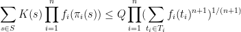
 is the quantity
 is the set of all tuples
  such that
  for
for  . When
  , the inequality reads

 the inequality reads

 , the existing proofs require the “tensor power trick” in order to reduce to the case when the
  are step functions (in which case the inequality can be proven elementarily, as discussed in the above paper of Carbery).
 and
and  for some functions
  and
and  . If we take logarithms in the inequality to be proven and apply Lemma
 ![\displaystyle \sup_X {\bf E} k(X) + \sum_{i=1}^n g_i(\pi_i(X)) + {\bf H}[X]](https://s0.wp.com/latex.php?latex=%5Cdisplaystyle++%5Csup_X+%7B%5Cbf+E%7D+k%28X%29+%2B+%5Csum_%7Bi%3D1%7D%5En+g_i%28%5Cpi_i%28X%29%29+%2B+%7B%5Cbf+H%7D%5BX%5D+&bg=ffffff&fg=000000&s=0&c=20201002)
![\displaystyle \leq \frac{1}{n+1} \sup_{(X_0,\dots,X_n)} {\bf E} k(X_0)+\dots+k(X_n) + {\bf H}[X_0,\dots,X_n]](https://s0.wp.com/latex.php?latex=%5Cdisplaystyle++%5Cleq+%5Cfrac%7B1%7D%7Bn%2B1%7D+%5Csup_%7B%28X_0%2C%5Cdots%2CX_n%29%7D+%7B%5Cbf+E%7D+k%28X_0%29%2B%5Cdots%2Bk%28X_n%29+%2B+%7B%5Cbf+H%7D%5BX_0%2C%5Cdots%2CX_n%5D+&bg=ffffff&fg=000000&s=0&c=20201002)
![\displaystyle + \frac{1}{n+1} \sum_{i=1}^n \sup_{Y_i} (n+1) {\bf E} g_i(Y_i) + {\bf H}[Y_i]](https://s0.wp.com/latex.php?latex=%5Cdisplaystyle++%2B+%5Cfrac%7B1%7D%7Bn%2B1%7D+%5Csum_%7Bi%3D1%7D%5En+%5Csup_%7BY_i%7D+%28n%2B1%29+%7B%5Cbf+E%7D+g_i%28Y_i%29+%2B+%7B%5Cbf+H%7D%5BY_i%5D&bg=ffffff&fg=000000&s=0&c=20201002)
 range over tuples of random variables taking values in
  range over random variables taking values in
  . Comparing the suprema, the claim now reduces to
 , where each
 ![\displaystyle {\bf H}[X_0,\dots,X_n] = (n+1) {\bf H}[X]](https://s0.wp.com/latex.php?latex=%5Cdisplaystyle++%7B%5Cbf+H%7D%5BX_0%2C%5Cdots%2CX_n%5D+%3D+%28n%2B1%29+%7B%5Cbf+H%7D%5BX%5D+&bg=ffffff&fg=000000&s=0&c=20201002)
![\displaystyle - {\bf H}[\pi_1(X)] - \dots - {\bf H}[\pi_n(X)].](https://s0.wp.com/latex.php?latex=%5Cdisplaystyle+-+%7B%5Cbf+H%7D%5B%5Cpi_1%28X%29%5D+-+%5Cdots+-+%7B%5Cbf+H%7D%5B%5Cpi_n%28X%29%5D.&bg=ffffff&fg=000000&s=0&c=20201002)
 . When
  . Now suppose that
  , and the claim has already been proven for
  , thus one has already obtained a tuple
  with each
  having the same distribution as
 ![\displaystyle {\bf H}[X_0,\dots,X_{n-1}] = n {\bf H}[X] - {\bf H}[\pi_1(X)] - \dots - {\bf H}[\pi_{n-1}(X)].](https://s0.wp.com/latex.php?latex=%5Cdisplaystyle++%7B%5Cbf+H%7D%5BX_0%2C%5Cdots%2CX_%7Bn-1%7D%5D+%3D+n+%7B%5Cbf+H%7D%5BX%5D+-+%7B%5Cbf+H%7D%5B%5Cpi_1%28X%29%5D+-+%5Cdots+-+%7B%5Cbf+H%7D%5B%5Cpi_%7Bn-1%7D%28X%29%5D.&bg=ffffff&fg=000000&s=0&c=20201002)
 has the same distribution as
  . For each value
  attained by
  and
and  and
and  respectively, and then concatenate them to form a tuple
  a further copy of
  . One can the use the
 ![\displaystyle {\bf H}[X_0,\dots,X_n] = {\bf H}[\pi_n(X_n)] + {\bf H}[X_0,\dots,X_n| \pi_n(X_n)]](https://s0.wp.com/latex.php?latex=%5Cdisplaystyle++%7B%5Cbf+H%7D%5BX_0%2C%5Cdots%2CX_n%5D+%3D+%7B%5Cbf+H%7D%5B%5Cpi_n%28X_n%29%5D+%2B+%7B%5Cbf+H%7D%5BX_0%2C%5Cdots%2CX_n%7C+%5Cpi_n%28X_n%29%5D&bg=ffffff&fg=000000&s=0&c=20201002)
![\displaystyle = {\bf H}[\pi_n(X_n)] + {\bf H}[X_0,\dots,X_{n-1}| \pi_n(X_n)] + {\bf H}[X_n| \pi_n(X_n)]](https://s0.wp.com/latex.php?latex=%5Cdisplaystyle++%3D+%7B%5Cbf+H%7D%5B%5Cpi_n%28X_n%29%5D+%2B+%7B%5Cbf+H%7D%5BX_0%2C%5Cdots%2CX_%7Bn-1%7D%7C+%5Cpi_n%28X_n%29%5D+%2B+%7B%5Cbf+H%7D%5BX_n%7C+%5Cpi_n%28X_n%29%5D+&bg=ffffff&fg=000000&s=0&c=20201002)
![\displaystyle = {\bf H}[\pi_n(X)] + {\bf H}[X_0,\dots,X_{n-1}| \pi_n(X_{n-1})] + {\bf H}[X_n| \pi_n(X_n)]](https://s0.wp.com/latex.php?latex=%5Cdisplaystyle++%3D+%7B%5Cbf+H%7D%5B%5Cpi_n%28X%29%5D+%2B+%7B%5Cbf+H%7D%5BX_0%2C%5Cdots%2CX_%7Bn-1%7D%7C+%5Cpi_n%28X_%7Bn-1%7D%29%5D+%2B+%7B%5Cbf+H%7D%5BX_n%7C+%5Cpi_n%28X_n%29%5D+&bg=ffffff&fg=000000&s=0&c=20201002)
![\displaystyle = {\bf H}[\pi_n(X)] + ({\bf H}[X_0,\dots,X_{n-1}] - {\bf H}[\pi_n(X_{n-1})])](https://s0.wp.com/latex.php?latex=%5Cdisplaystyle++%3D+%7B%5Cbf+H%7D%5B%5Cpi_n%28X%29%5D+%2B+%28%7B%5Cbf+H%7D%5BX_0%2C%5Cdots%2CX_%7Bn-1%7D%5D+-+%7B%5Cbf+H%7D%5B%5Cpi_n%28X_%7Bn-1%7D%29%5D%29+&bg=ffffff&fg=000000&s=0&c=20201002)
![\displaystyle + ({\bf H}[X_n] - {\bf H}[\pi_n(X_n)])](https://s0.wp.com/latex.php?latex=%5Cdisplaystyle+%2B+%28%7B%5Cbf+H%7D%5BX_n%5D+-+%7B%5Cbf+H%7D%5B%5Cpi_n%28X_n%29%5D%29+&bg=ffffff&fg=000000&s=0&c=20201002)
![\displaystyle ={\bf H}[X_0,\dots,X_{n-1}] + {\bf H}[X_n] - {\bf H}[\pi_n(X_n)]](https://s0.wp.com/latex.php?latex=%5Cdisplaystyle++%3D%7B%5Cbf+H%7D%5BX_0%2C%5Cdots%2CX_%7Bn-1%7D%5D+%2B+%7B%5Cbf+H%7D%5BX_n%5D+-+%7B%5Cbf+H%7D%5B%5Cpi_n%28X_n%29%5D&bg=ffffff&fg=000000&s=0&c=20201002)
 and
and  be sequences of real numbers indexed by natural numbers
  , with
  non-increasing and
  non-negative. Suppose also that
  for all
  . Then
  for all
  .
.
 is non-negative, and
  by hypothesis, we have
 the left-hand side is at least
  , giving the claim.
 . With a little bit of pen and paper effort, I obtained


 (denoted
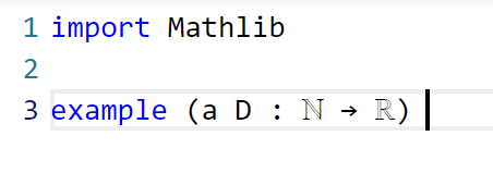


 , and also “


 , I (together with
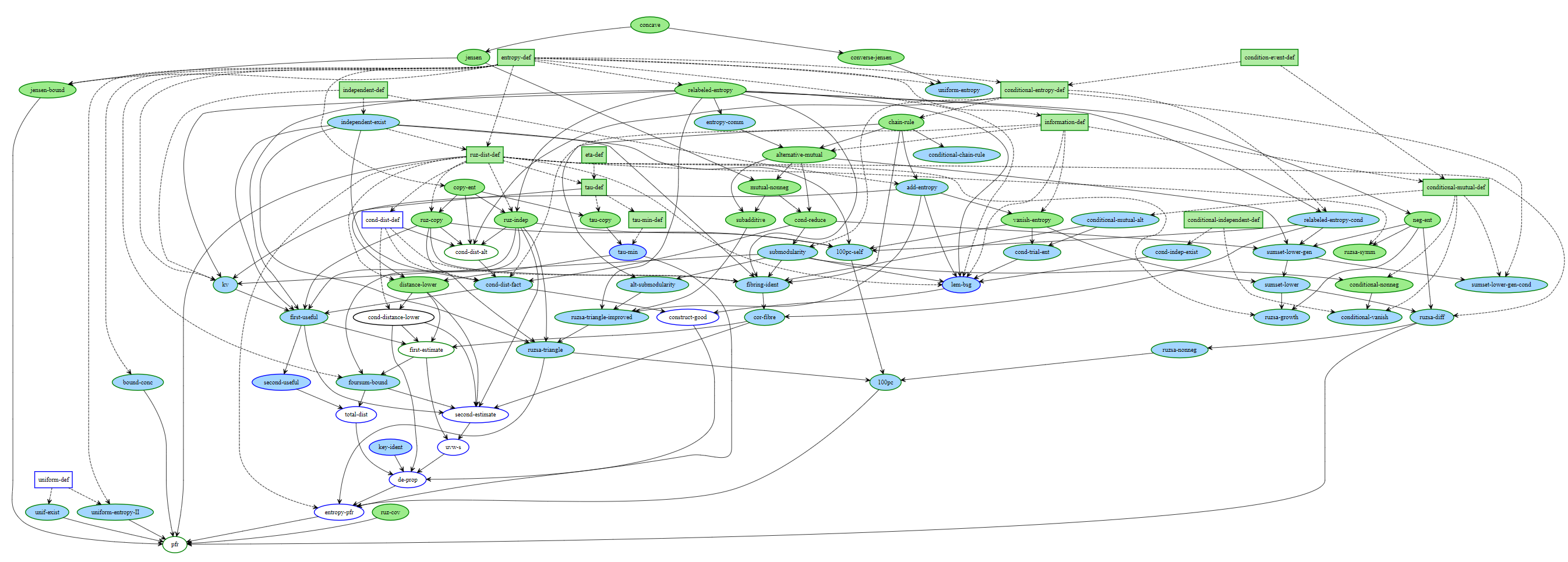


 is a finite elementary abelian group of order
  (this is how we have chosen to formalize the finite field vector spaces
  ), that
  is a non-empty subset of
  less than
  times the cardinality of
  of a subgroup
  of
of  of cardinality at most
  .
. 

![d[X; Y]](https://s0.wp.com/latex.php?latex=d%5BX%3B+Y%5D&bg=ffffff&fg=545454&s=0&c=20201002) refers to something called the entropic Ruzsa distance between
refers to something called the entropic Ruzsa distance between  and
and  , which is something that is defined
![H[X]](https://s0.wp.com/latex.php?latex=H%5BX%5D&bg=ffffff&fg=545454&s=0&c=20201002) , by the way, refers to the
, by the way, refers to the ![|H[X] - H[Y]|](https://s0.wp.com/latex.php?latex=%7CH%5BX%5D+-+H%5BY%5D%7C&bg=ffffff&fg=545454&s=0&c=20201002) is clearly non-negative! (There is a factor of
is clearly non-negative! (There is a factor of 
 are introduced at an earlier stage in the Lean file; again, we will ignore this point for the ensuing discussion.) Meanwhile, Lemma 3.13 is

 to
to 
![0 \leq 2 d[X;Y]](https://s0.wp.com/latex.php?latex=0+%5Cleq+2+d%5BX%3BY%5D&bg=ffffff&fg=545454&s=0&c=20201002) implies
implies ![0 \leq d[X,Y]](https://s0.wp.com/latex.php?latex=0+%5Cleq+d%5BX%2CY%5D&bg=ffffff&fg=545454&s=0&c=20201002) , and the other to show that
, and the other to show that 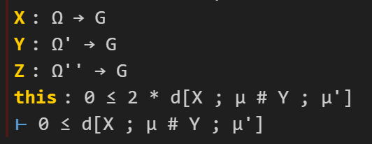


![|H[X]-H[Y]| \leq 2 d[X;Y]](https://s0.wp.com/latex.php?latex=%7CH%5BX%5D-H%5BY%5D%7C+%5Cleq+2+d%5BX%3BY%5D&bg=ffffff&fg=545454&s=0&c=20201002) (which I will call “h”), and then to deduce the previous goal
(which I will call “h”), and then to deduce the previous goal  . For the first, I know I should invoke the lemma “diff_ent_le_rdist” that is encoding Lemma 3.11. One way to do this is to try the tactic “exact?”, which will automatically search to see if the goal can already be deduced immediately from an existing lemma. It reports:


![0 \leq |H[X] - H[Y]|](https://s0.wp.com/latex.php?latex=0+%5Cleq+%7CH%5BX%5D+-+H%5BY%5D%7C&bg=ffffff&fg=545454&s=0&c=20201002) :
:
 to give the desired goal, and it works!
 relation rather than the
  relation, but in Lean the assertions
  and
and  are “
are “


 in the above two lemmas to make them completely true, but this is something that should emerge organically as the formalization process continues.)
 be such that
  translates of a subspace
  of cardinality at most
  for any
  (assuming that say
  to avoid some degeneracies as
  approaches
  , which is not the difficult case of the conjecture). The conjecture (with
  ) has a number of equivalent forms; see this
  theorem are now polynomial in nature (although we did not try to optimize the constant).
 ), but can be improved even further with additional effort (our current argument, for instance, allows one to replace it with
  , but we decided to state our result using integer exponents instead).
 . Indeed, suppose for instance that one could show that every set
  . One measure of commensurability, for instance, might be the Ruzsa distance
  , which one might hope to control by
  . Then one could iterate this procedure until doubling constant dropped below say
  , at which point the conjecture is known to hold (there is an elementary argument that if
  is in fact a subspace of
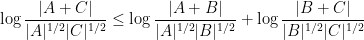
 ) of a large subspace
  for a “typical”
  . For instance, if
  subset of
  random translates of a medium-sized subspace
  has doubling constant
  . On the other hand, by using the projection map
  defined by
  , we see that
  , with fibres
  being essentially a copy of
  , times the doubling constant of a typical fibre
  and
and  is the entropic doubling constant
  , where
  are independent copies of
  is a homomorphism, one then has what we call the fibring inequality
 is defined as


 of itself, and using the addition map
  for
for  , we obtain in particular that
 is determined by
  once one fixes
  )
) 
 , then at least one of
  or
or  will be less than or equal to
  . This is the entropy analogue of at least one of (i) or (ii) improving, or at least not degrading the doubling constant, although there are some minor technicalities involving how one deals with the conditioning to
  ,
,  , and “depolarise” the induction hypothesis to deal with distances
  between pairs of random variables

 . This leads (modulo some technicalities) to the following interesting conclusion: if neither (i) nor (ii) leads to an improvement in the entropic doubling constant, then
  are conditionally independent relative to
  . This situation (or an approximation to this situation) is what we refer to in the paper as the “endgame”.

 has exactly the same distribution; in particular, the entropic doubling constant here is zero, which is certainly a reduction in the doubling constant.

Recent Comments